10 Gravitational Field of an Axially Symmetric System

In order to investigate the possibility of a physical system radiating gravitational waves, 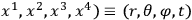it seems desirable to choose a simple system, one with axial symmetry. If the field of such a system is described by means of a spherical polar coordinate system, ( , then by a suitable choice of coordinates one can satisfy two conditions:

(a) The metric tensor is independent of the angle .

(b) It is diagonal.

If one writes down the field equations in the empty space surrounding the system

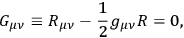
one obtains a set of 7 equations (since vanishes identically if one index is equal to 3) for the 4 diagonal components of . Among these there exist 3 identities (the Bianchi identities, except for the one with index 3).

The field equations are non-linear and difficult to solve. It is proposed to investigate them by the method of successive approximations. As a beginning, the first approximation can be calculated. Let us write the line element in the form

where , , , and are regarded as small of the first order. The linear approximation of the field equations has the following form (indexes denoting partial differentiation):

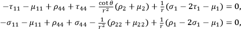
From these equations it is possible to derive the wave equation for ,

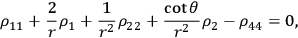
and to express the other unknowns in terms of the solution for .

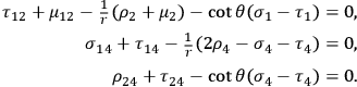
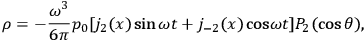
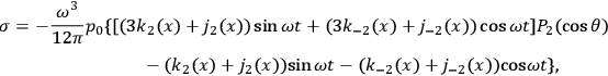
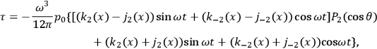
If we represent the radiating system by a quadrupole mass moment , then the solution describing outgoing monochromatic waves can be written in terms of the frequency and the amplitude of the moment 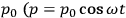) as follows:

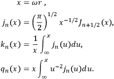
Here

It is planned to use this solution as the starting point for a more accurate calculation. The interesting question, of course, is whether the exact equations have a solution going over into the above for sufficiently weak fields.

***

J. N. GOLDBERG presented an approximation method for high velocities. The obvious one is a mass expansion of the gravitational field. In the first approximation there is no acceleration of the particles, which are represented by singularities. This situation differs from the corresponding case in electromagnetic theory. The reason for this is that the electromagnetic field is described by a vector potential whereas the gravitational field is tensor in character. In the E.I.H. method, the motion of the particles is determined by certain consistency conditions in the form of surface integrals each of which contains two terms. One of these is the time derivative of an expression which is linear in the first derivatives of the potentials, the other is quadratic in the first derivatives of the potentials. Therefore, in each order the surface integrals place restrictions on the solutions of lower order. These restrictions may be relaxed by adding appropriate poles and dipoles in the lower orders. The requirement that the sum of the dipoles added must vanish leads to the equations of motion. However, since we do not discriminate against the time in the mass expansion, the surface integral conditions must be satisfied in the same order as the corresponding field equations. This situation is very unsatisfactory. The surface integrals, however, are related to the Bianchi identities. Instead of the surface integral conditions, one can require that the Bianchi identities be satisfied everywhere, even across the singularities. In this manner one can obtain higher order equations of motion from the lower order field equations both in the E.I.H. method and in the mass expansion.

TONNELAT: The starting point of the non-symmetric unified field theory is usually the invariant density:

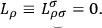
in which is the Ricci tensor built from an arbitrary affine connection . The variations , lead to the field equations. However, if one tries to apply the Einstein, Infeld, Hoffmann method to these equations, one obtains merely the results of general relativity, and one does not obtain the equations for a charged particle. This result stems from the condition

which is imposed by the theory.

To avoid this situation, one can start from an affine connection with vanishing torque

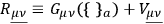
Lagrange multipliers are needed in the variations of because the 64 are not independent and, moreover, the vector related to the torque is introduced. In this case, one obtains

Introducing the metric

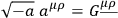
one obtains

with

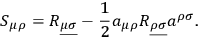
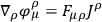
Setting

defines a tensor whose divergence gives a Lorentz force. This tensor plays in the field equations the role of a Maxwell tensor and leads, with the use of an extension of the Einstein, Infeld, Hoffmann method, to a Coulomb force.